Discrete Fourier Transform by Hand ✍️

In signal processing, the Discrete Fourier Transform (DFT) is no doubt the most important method. But the math involved is extremely complex, literally, involving a summation over a complex number term e^(-iwt), where e is the Euler number, i is the imaginary unit, w is the angular frequency, and t is time.

I developed this exercise to demonstrate that underneath such complexity, DFT is just a series of matrix multiplications you can calculate by hand. ✍️ Once you see that, it should not surprise you that a deep neural network, which is also a series of matrix multiplications, with activation functions in-between, can learn to perform DFT to process and analyze signals so effectively.

💡 Learned vs. Fixed: U-Net learns its filters from data to process a signal in the spatial domain. The DFT is the classical opposite, a fixed transform, designed by hand rather than learned, that views the same signal in the frequency domain as a combination of cosine waves.

How does DFT work?

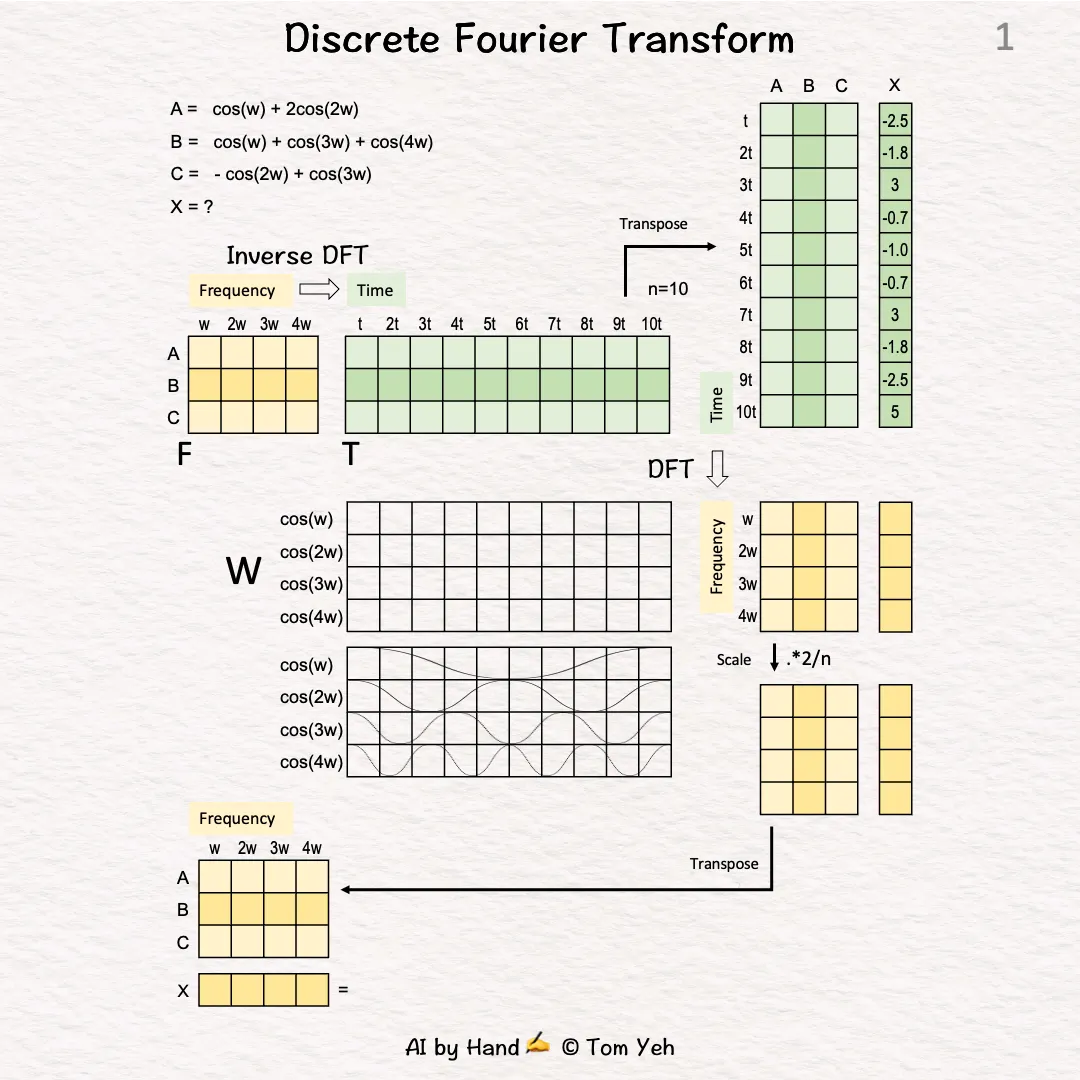
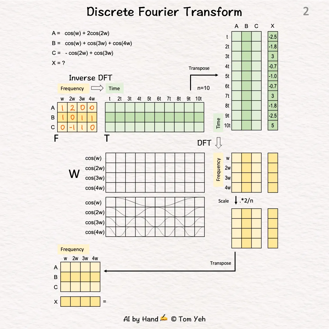
• Signals A, B, and C in the 🟧 frequency domain:

• A = cos(w) + 2cos(2w)

• B = cos(w) + cos(3w) + cos(4w)

• C = -cos(2w) + cos(3w)

• Each signal is a weighed sum of four cosine waves at frequencies 1w, 2w, 3w, and 4w.

• We will apply Inverse DFT to convert the signals to time domain representations, and then demonstrate DFT can convert back to their original frequency domain representations.

• Signal X in the 🟩 time domain. X is sampled at 10 time points 1t, 2t, …, 10t:

• X = [-2.5, -1.8, 3, -0.7, -1.0, -0.7, 3, -1.8, -2.5, 5]

• Suppose X is also a weighted sum of the same four cosine waves, but we don’t already know their weights. We will apply DFT to discover them.

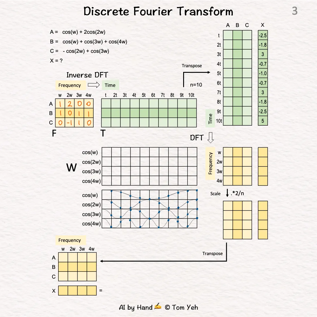
• Sample from the continuous cosine waves at discrete time points 1t, 2t, 3t, to 10t.