Why Backprop Goes Backward

The usual explanation of backpropagation (Rumelhart et al., 1986), the algorithm used to train neural networks, is that it is propagating errors for each node backwards. But when I first learned about the algorithm, I had a question that I could not find answered directly: why does it have to go backwards? A neural network is just a composite function, and we know how to compute the derivatives of composite functions using the chain rule. Why don’t we just compute the gradient in a forward pass? I found that answering this question strengthened my understanding of backprop.

I will assume the reader broadly understands neural networks and gradient descent and even has some familiarity with backprop. I’ll first setup backprop with some useful concepts and notation and then explain why a forward propagation algorithm is supoptimal.

Setup

Recall that the goal of backprop is to efficiently compute $\partial f / \partial \theta_i$

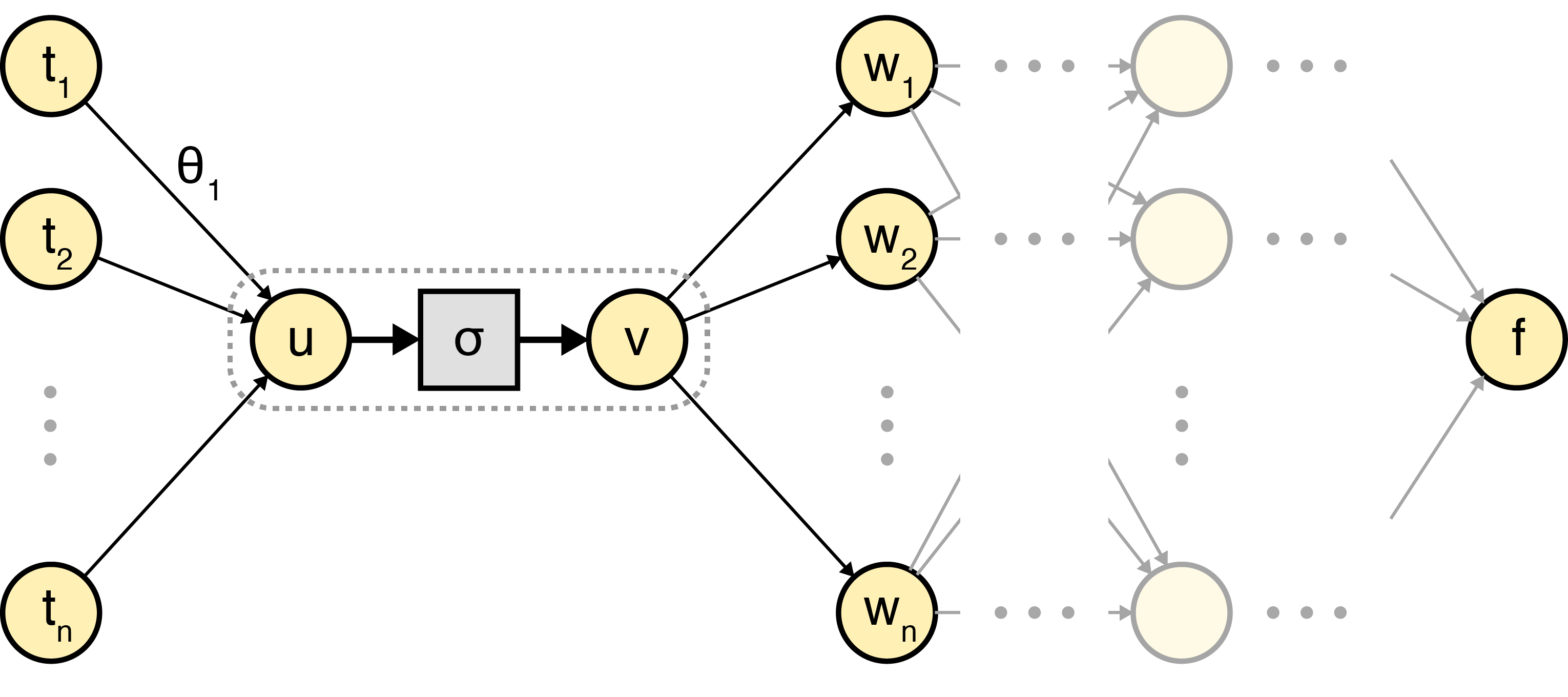
To be clear, the node $v$ refers to the output value of the node after passing the weighted sum of its inputs through an activation function $\sigma$, i.e.:

$\begin🔥 u &= \theta_1 t_1 + \theta_2 t_2 + \dots + \theta_n t_n \\ v &= \sigma(u) \end⚡$

Note that in a typical diagram, $u$, $\sigma$, and $v$ would all be a single node, denoted by the dashed line. In my mind, the most important observation needed to understand backprop is this: most of computing $\partial f / \partial \theta_1$

$\frac🔥⚡ = \frac{\partial f}{\partial v} \frac{\partial v}{\partial u} \frac{\partial u}{\partial \theta_1}$

We can compute $\partial v / \partial u$ analytically; it just depends on the definition of $\sigma$. And we know that $\partial u / \partial \theta_1 = t_1$

The challenge with computing $\partial f / \partial v$ is that downstream nodes depend on the value of $v$. Thankfully, the multivariable chain rule has the answer. Given a multivariable function $g(w_1, w_2, \dots, w_m)$

$\frac{\partial g}{\partial v} = \frac{\partial}{\partial v} g(w_1(v), w_2(v), \dots, w_m(v)) = \sum_{j} \frac{\partial g}{\partial w_j} \frac{\partial w_j}{\partial v}$

So we can compute $\partial f / \partial \theta_i$

Repeated terms

We want a forward propagating algorithm that can compute the partial derivative $\partial f / \partial \theta_i$

$\frac{\partial f}{\partial \theta_i} = \frac{\partial f}{\partial v} \frac{\partial v}{\partial \theta_i}$

Note that I’ve dropped the intermediate variable $u$ for ease of notation. To design our forward propagating algorithm, let’s formalize an important fact: in a directed computational graph in which node $b$ depends upon node $a$, it is impossible to compute $\partial b / \partial a$ at any point before node $b$:

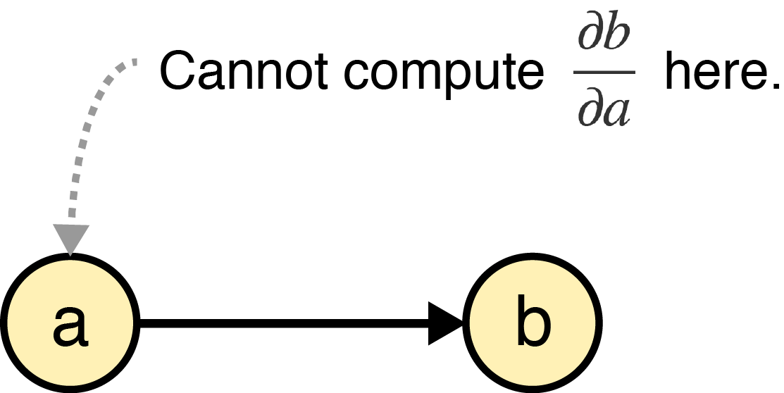
This claim should be obvious. If our computational graph represents a function $f(a) = b$

In our setup, for every downstream node $w_j$

$\frac{\partial f}{\partial \theta_i} = \Big( \sum_{j} \frac{\partial f}{\partial w_j} \underbrace{\frac{\partial w_j}{\partial v}}_{\text{Compute on $w_j$}} \Big) \overbrace{\frac{\partial v}{\partial \theta_i}}^{\text{Pass forward}}$

We can see that such an algorithm blows up computationally because we’re forward propagating the same message many times over. For example, if we want to compute $\partial f / \partial \theta_i$

$\begin{aligned} \frac{\partial f}{\partial \theta_i} = \overbrace{ \Big( \sum_{j} \Big( \sum_{k} \frac{\partial f}{\partial z_k} \frac{\partial z_k}{\partial w_j} \Big) \frac{\partial w_j}{\partial v} \Big)}^{\text{Repeated terms}} \color{#11accd}{ \frac{\partial v}{\partial \theta_i} } \\ \frac{\partial f}{\partial \theta_k} = \Big( \sum_{j} \Big( \sum_{k} \frac{\partial f}{\partial z_k} \frac{\partial z_k}{\partial w_j} \Big) \frac{\partial w_j}{\partial v} \Big) \color{#bc2612}{ \frac{\partial v}{\partial \theta_k} } \end{aligned}$

Here is a diagram of message passing the repeated terms:

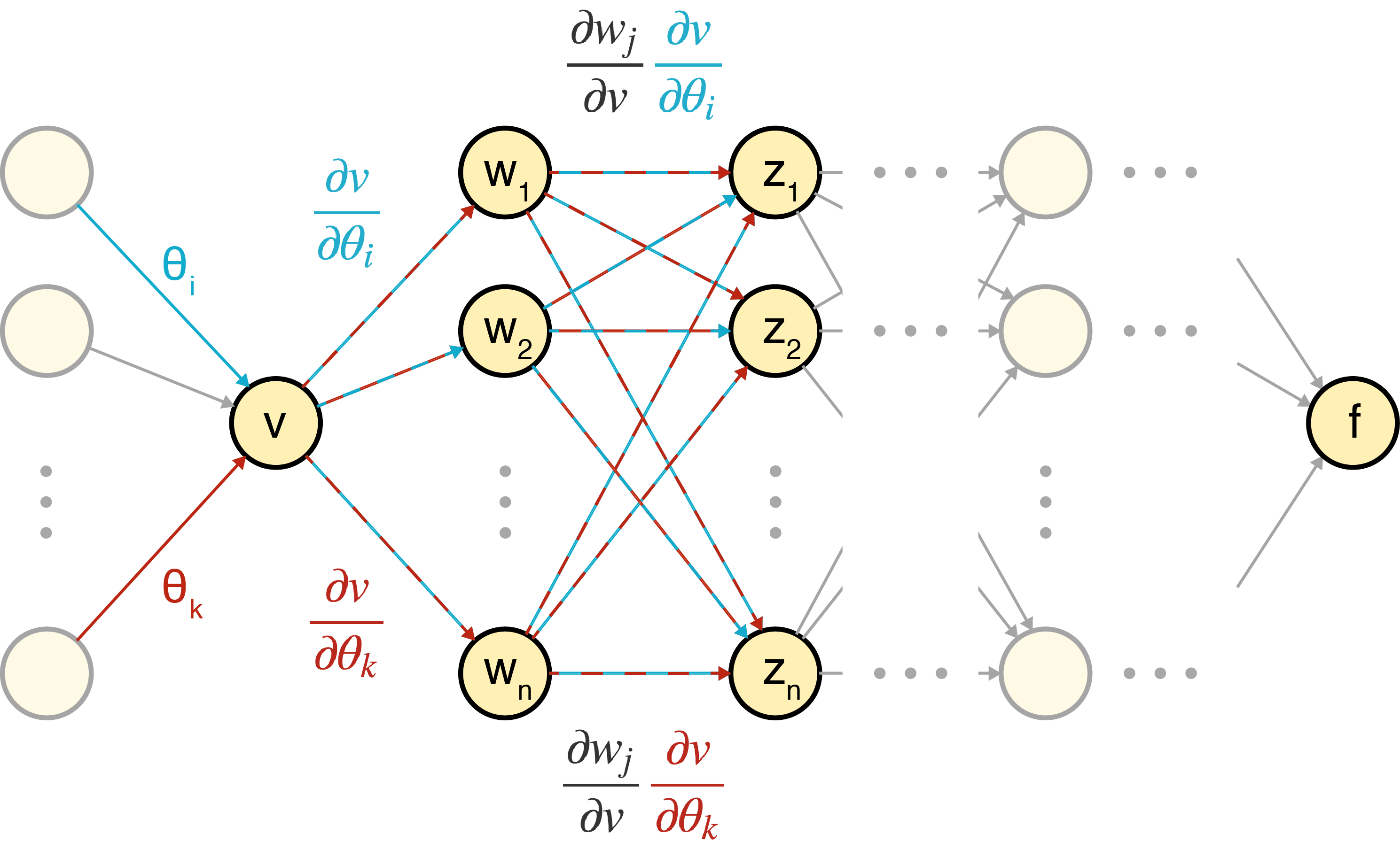
I think the above diagram is the lynchpin in understanding why backprop goes backwards. This is the key insight: if we already had access to downstream terms, for example $\partial w_j / \partial v$

A backward pass

I hope this explanation it clarifies how you might get to backprop from first principles trying to compute derivatives in a directed acyclic graph. On a given node $b$ that depends on a node $a$, we simply message pass $\partial b / \partial a$ back to $a$. The multivariable chain rule helps prove the correctness of backprop. For any node $v$ with downstream weights $w_j$

$\frac{\partial f}{\partial v} = \sum_{j} \frac{\partial f}{\partial w_j} \frac{\partial w_j}{\partial v}$

Once you understand the main computational problem backprop solves, I think the standard explanation of backpropagating errors makes much more sense. This process is can be viewed as a solution to a kind of credit assignment problem: each node tells its upstream neighbors what they did wrong. But the reason the algorithm works this way is because a naive, forward propagating solution would have quadratic runtime in the number of nodes.