LLM Transformer Model Visually Explained

Transformer is a neural network architecture that has fundamentally changed the approach to
Artificial Intelligence. Transformer was first introduced in the seminal paper
“Attention is All You Need”
in 2017 and has since become the go-to architecture for deep learning models, powering text-generative
models like OpenAI’s GPT, Meta’s Llama, and Google’s
Gemini. Beyond text, Transformer is also applied in
audio generation,
image recognition,
protein structure prediction, and even
game playing, demonstrating its versatility across numerous domains.

Fundamentally, text-generative Transformer models operate on the principle of next-token prediction: given a text prompt from the user, what is the
most probable next token (a word or part of a word) that will follow this input? The core
innovation and power of Transformers lie in their use of self-attention mechanism, which allows
them to process entire sequences and capture long-range dependencies more effectively than previous
architectures.

GPT-2 family of models are prominent examples of text-generative Transformers. Transformer
Explainer is powered by the
GPT-2
(small) model which has 124 million parameters. While it is not the latest or most powerful Transformer
model, it shares many of the same architectural components and principles found in the current
state-of-the-art models making it an ideal starting point for understanding the basics.

Every text-generative Transformer consists of these three key components:

1. Embedding: Text input is divided into smaller units
   called tokens, which can be words or subwords. These tokens are converted into numerical
   vectors called embeddings, which capture the semantic meaning of words.
2. Transformer Block is the fundamental building block of
   the model that processes and transforms the input data. Each block includes:
   • Attention Mechanism, the core component of the Transformer block. It
     allows tokens to communicate with other tokens, capturing contextual information and
     relationships between words.
   • MLP (Multilayer Perceptron) Layer, a feed-forward network that operates
     on each token independently. While the goal of the attention layer is to route
     information between tokens, the goal of the MLP is to refine each token’s
     representation.
3. Output Probabilities: The final linear and softmax
   layers transform the processed embeddings into probabilities, enabling the model to make
   predictions about the next token in a sequence.

Embedding

Let’s say you want to generate text using a Transformer model. You add the prompt like this
one: “Data visualization empowers users to”. This input needs to be converted
into a format that the model can understand and process. That is where embedding comes in: it
transforms the text into a numerical representation that the model can work with. To convert a
prompt into embedding, we need to 1) tokenize the input, 2) obtain token embeddings, 3) add
positional information, and finally 4) add up token and position encodings to get the final
embedding. Let’s see how each of these steps is done.

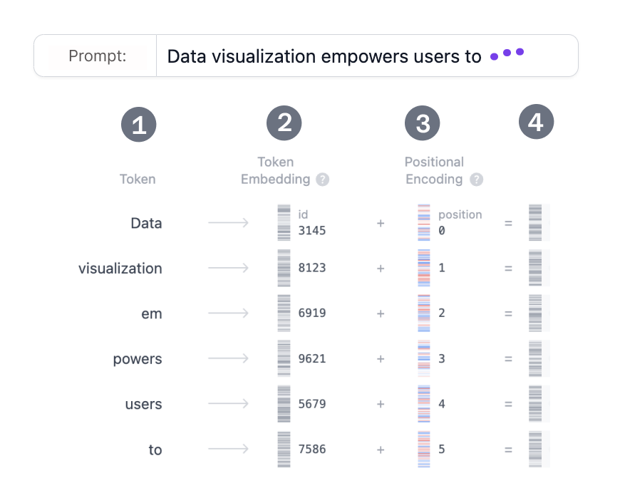
Figure 1. Expanding the Embedding layer view, showing how the
input prompt is converted to a vector representation. The process involves
(1) Tokenization, (2) Token Embedding, (3) Positional Encoding,
and (4) Final Embedding.

Transformer Block

The core of the Transformer’s processing lies in the Transformer block, which comprises
multi-head self-attention and a Multi-Layer Perceptron layer. Most models consist of multiple
such blocks that are stacked sequentially one after the other. The token representations
evolve through layers, from the first block to the last one, allowing the model to build up an
intricate understanding of each token. This layered approach leads to higher-order
representations of the input. The GPT-2 (small) model we are examining consists of 12 such blocks.

Multi-Head Self-Attention

The self-attention mechanism enables the model to capture relationships among tokens in a
sequence, so that each token’s representation is influenced by the others. Multiple attention
heads allow the model to consider these relationships from different perspectives; for
example, one head may capture short-range syntactic links while another tracks broader
semantic context. In the following section, we will walk through how multi-head self-attention
is computed step by step.

Step 1: Query, Key, and Value Matrices

$$QKV_💬 = ( \sum_⚡^💬 \text⚡_{i,d} \cdot \text{Weights}_{d,j}) + \text{Bias}_j$$

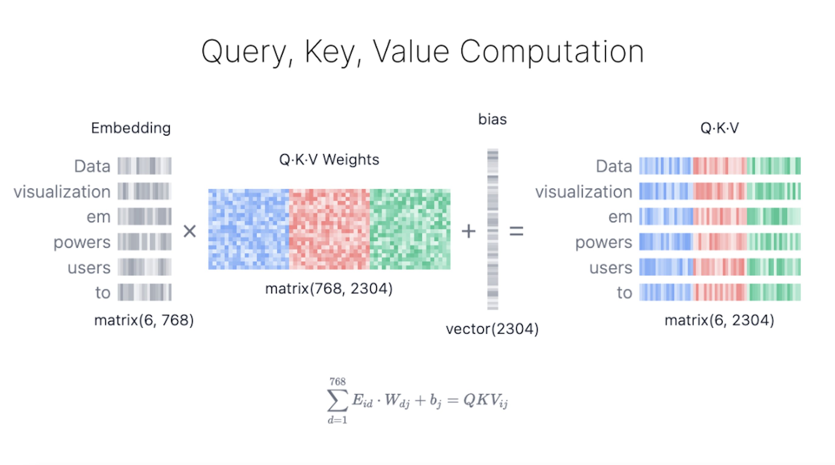
Figure 2. Computing Query, Key, and Value matrices from the
original embedding.

Each token’s embedding vector is transformed into three vectors:
Query (Q),
Key (K), and
Value (V). These vectors are derived by multiplying the input
embedding matrix with learned weight matrices for
Q,
K, and
V. Here’s a web search analogy to help us build some intuition
behind these matrices:

• Query (Q) is the search text you type in the
  search engine bar. This is the token you want to
  “find more information about”.
• Key (K) is the title of each web page in the search
  result window. It represents the possible tokens the query can attend to.
• Value (V) is the actual content of web pages shown.
  Once we matched the appropriate search term (Query) with the relevant results (Key), we want
  to get the content (Value) of the most relevant pages.

By using these QKV values, the model can calculate attention scores, which determine how
much focus each token should receive when generating predictions.

Step 3: Masked Self-Attention

In each head, we perform masked self-attention calculations. This mechanism allows the model
to generate sequences by focusing on relevant parts of the input while preventing access to
future tokens.

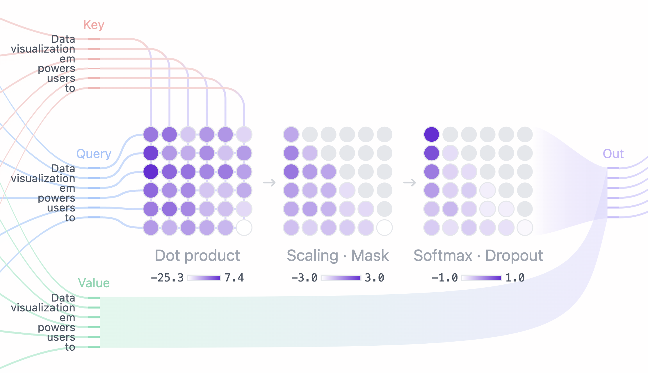
Figure 3. Using Query, Key, and Value matrices to calculate
masked self-attention.

• Dot Product: The dot product of
  Query
  and Key matrices determines the
  attention score, producing a square matrix that reflects the relationship
  between all input tokens.
• Scaling · Mask: The attention scores are scaled and a mask is applied to
  the upper triangle of the attention matrix to prevent the model from accessing future
  tokens, setting these values to negative infinity. The model needs to learn how to predict
  the next token without “peeking” into the future.
• Softmax · Dropout: After masking and scaling, the attention scores are
  converted into probabilities by the softmax operation, then optionally regularized with
  dropout. Each row of the matrix sums to one and indicates the relevance of every other
  token to the left of it.

MLP: Multi-Layer Perceptron

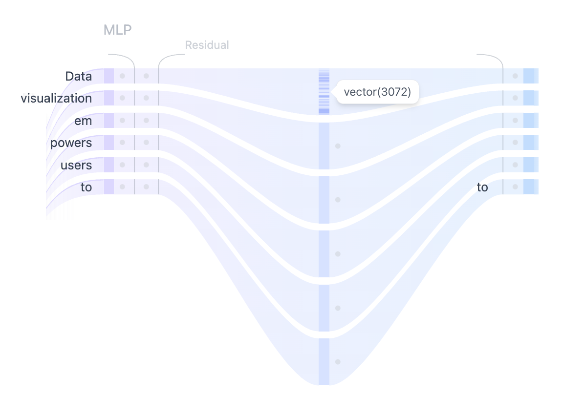
Figure 4. Using MLP layer to project the self-attention
representations into higher dimensions to enhance the model’s representational capacity.

After the multiple heads of self-attention capture the diverse relationships between the input
tokens, the concatenated outputs are passed through the Multilayer Perceptron (MLP) layer to
enhance the model’s representational capacity. The MLP block consists of two linear
transformations with a GELU activation function in between.

The first linear transformation expands the dimensionality of the input four-fold from 768
to
3072. This expansion step allows the model to project the token representations
into a higher-dimensional space, where it can capture richer and more complex patterns that
may not be visible in the original dimension.

The second linear transformation then reduces the dimensionality back to the original size of 768.This compression step brings the representations back to a manageable size while retaining
the useful nonlinear transformations introduced in the expansion step.

Unlike the self-attention mechanism, which integrates information across tokens, the MLP
processes tokens independently and simply maps each token representation from one space to
another, enriching the overall model capacity.

Output Probabilities

After the input has been processed through all Transformer blocks, the output is passed
through the final linear layer to prepare it for token prediction. This layer projects the
final representations into a 50,257
dimensional space, where every token in the vocabulary has a corresponding value called
logit. Any token can be the next word, so this process allows us to simply rank
these tokens by their likelihood of being that next word. We then apply the softmax function
to convert the logits into a probability distribution that sums to one. This will allow us to
sample the next token based on its likelihood.

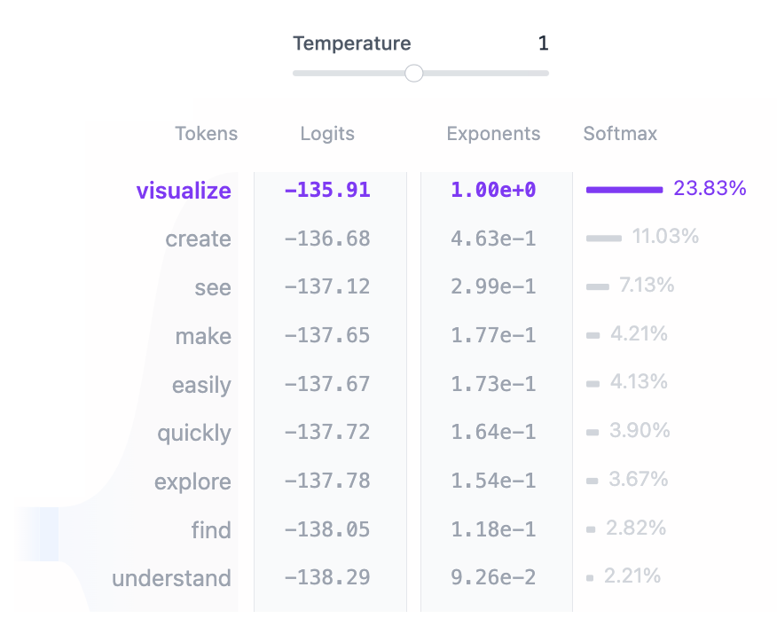
Figure 5. Each token in the vocabulary is assigned a
probability based on the model’s output logits. These probabilities determine the likelihood
of each token being the next word in the sequence.

The final step is to generate the next token by sampling from this distribution The temperature
hyperparameter plays a critical role in this process. Mathematically speaking, it is a very simple
operation: model output logits are simply divided by the
temperature:

• temperature = 1: Dividing logits by one has no effect on the softmax outputs.
• temperature < 1: Lower temperature makes the model more confident and
  deterministic by sharpening the probability distribution, leading to more predictable
  outputs.
• temperature > 1: Higher temperature creates a softer probability
  distribution, allowing for more randomness in the generated text – what some refer to as
  model “creativity”.

In addition, the sampling process can be further refined using top-k
and
top-p parameters:

• top-k sampling: Limits the candidate tokens to the top k tokens with the
  highest probabilities, filtering out less likely options.
• top-p sampling: Considers the smallest set of tokens whose cumulative
  probability exceeds a threshold p, ensuring that only the most likely tokens contribute
  while still allowing for diversity.

By tuning temperature, top-k, and top-p, you can
balance between deterministic and diverse outputs, tailoring the model’s behavior to your
specific needs.

Auxiliary Architectural Features

There are several auxiliary architectural features that enhance the performance of Transformer
models. While important for the model’s overall performance, they are not as important for
understanding the core concepts of the architecture. Layer Normalization, Dropout, and
Residual Connections are crucial components in Transformer models, particularly during the
training phase. Layer Normalization stabilizes training and helps the model converge faster.
Dropout prevents overfitting by randomly deactivating neurons. Residual Connections allows
gradients to flow directly through the network and helps to prevent the vanishing gradient
problem.

Transformer Explainer is built to be interactive and allows you to explore the inner workings
of the Transformer. Here are some of the interactive features you can play with:

• Input your own text sequence to see how the model processes it and predicts
  the next word. Explore attention weights, intermediate computations, and see how the final output
  probabilities are calculated.
• Use temperature slider to control the randomness of the model’s predictions.
  Explore how you can make the model output more deterministic or more creative by changing the
  temperature value.
• Select top-k and top-p sampling methods to adjust sampling behavior during inference.
  Experiment with different values and see how the probability distribution changes and influences
  the model’s predictions.
• Interact with attention maps to see how the model focuses on different tokens
  in the input sequence. Hover over tokens to highlight their attention weights and explore how
  the model captures context and relationships between words.

How is Transformer Explainer Implemented?

Transformer Explainer features a live GPT-2 (small) model running directly in the browser.
This model is derived from the PyTorch implementation of GPT by Andrej Karpathy’s
nanoGPT project
and has been converted to
ONNX Runtime
for seamless in-browser execution. The interface is built using JavaScript, with
Svelte
as a front-end framework and
D3.js
for creating dynamic visualizations. Numerical values are updated live following the user input.