blog | nworbmot:tombrown

The full set of technical assumptions, mostly leaning on the
Danish Energy Agency Technology Database, can be found here:

https://github.com/nworbmot/solar-battery-world/blob/main/defaults.csv

As well as the incremental energy cost for the lithium-ion batteries,
an inverter cost of 177 €/kW in 2030 and 66 €/kW in 2050 is also
included. The lithium-ion batteries have a round-trip efficiency of
96%.

The model is based on model.energy but without the hydrogen
storage. It is optimised with free backup generation for the final
10/5/1% then the costs are added back on top. This allows the user to
easily increase the investment or fuel cost for the backup, since this
is the most uncertain part of the costing.

To reproduce the optimisation on model.energy, choose the point
location in “Step 1”. Then for the technologies in “Step 3”, disable
wind and hydrogen storage. Under “Advanced settings” enable the
checkbox for “Dispatchable technology 1” and set both its overnight
cost and marginal cost to zero. To get (100-x)% solar-battery
coverage, i.e. limit the backup to x% coverage, put a dummy emissions
factor of 100 gCO₂/kWh_el on the backup, and then activate the
checkbox for the overall CO₂ limit and set the allowed emissions to x
gCO₂/kWh_el. The CO₂ emissions limit is being used as a proxy for
the overall backup fuel usage.

Once you have the optimisation result, you can add the backup costs
separately. For example, if the solar-battery system on its own costs
50 €/MWh for (100-x)% coverage, where x=10,5,1, then you add for the
backup per €/MWh (assuming enough backup capacity to cover the entire load):

investment cost * (annuity factor + FOM) / 8760 + fuel cost * x / efficiency

For the default back investment cost of 1 M€/MW, 25 year lifetime, 5% cost of capital, 3% yearly FOM, fuel cost of 30 €/MWh_th, efficiency 50% you get

1e6 * (0.071 + 0.03) / 8760 + 30*(x/100)/0.5 = (11.5 + 0.6x) €/MWh

If the investment cost rises to 2 M€/MW, the fixed part rises from
11.5 €/MWh to 23 €/MWh.

For x=10 with the original settings, you get a total 17.5 €/MWh
contribution from the backup.

If the fuel cost rises from 30 €/MWh to 50 €/MWh, the backup
contribution rises to (11.5 + x) = 21.5 €/MWh.

The sensitivity of the total cost to the fuel cost is directly tied to
x – the more solar and wind, the lower x and the less the fuel
dependency becomes.

To supply the full demand with these assumptions with a fuel cost of
30 €/MWh_th would cost (11.5 + 60) = 71.5 €/MWh, which is more
expensive in most locations that the solar-battery-fuel
system. However the cost of the backup fuel will vary by location
based on availability. If it rises to 60 €/MWh_th the full system
costs would rise to (11.5 + 120) = 131.5 €/MWh.

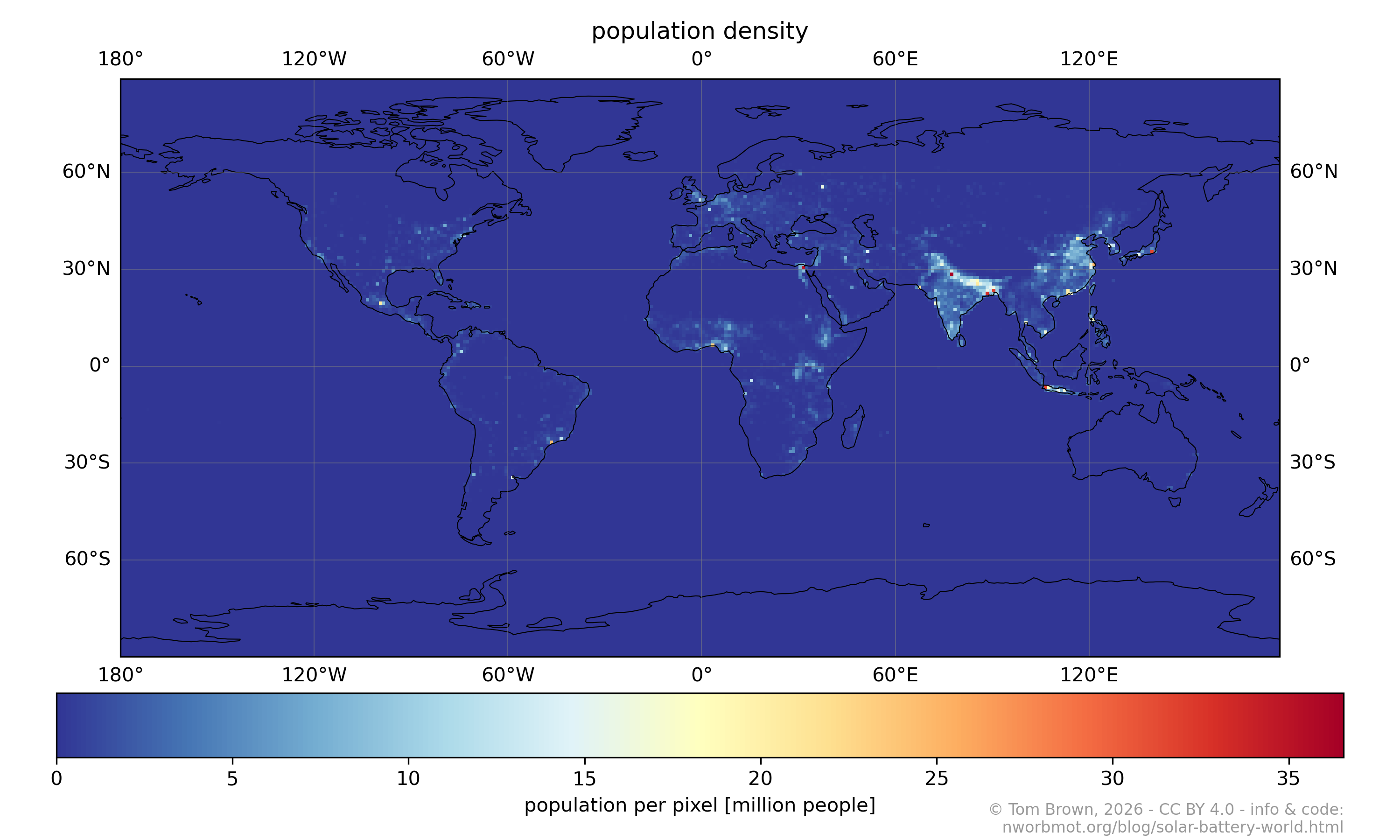
The calculations are carried out for the 9196 1° by 1° pixels that
contains more than 10,000 people, which is enough to include 99.86% of
the population.

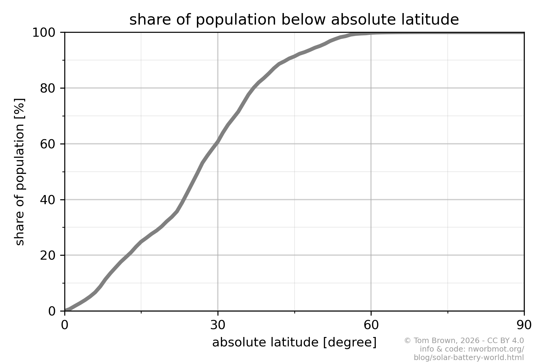
90% of the population lives within 45 degrees of the equator:

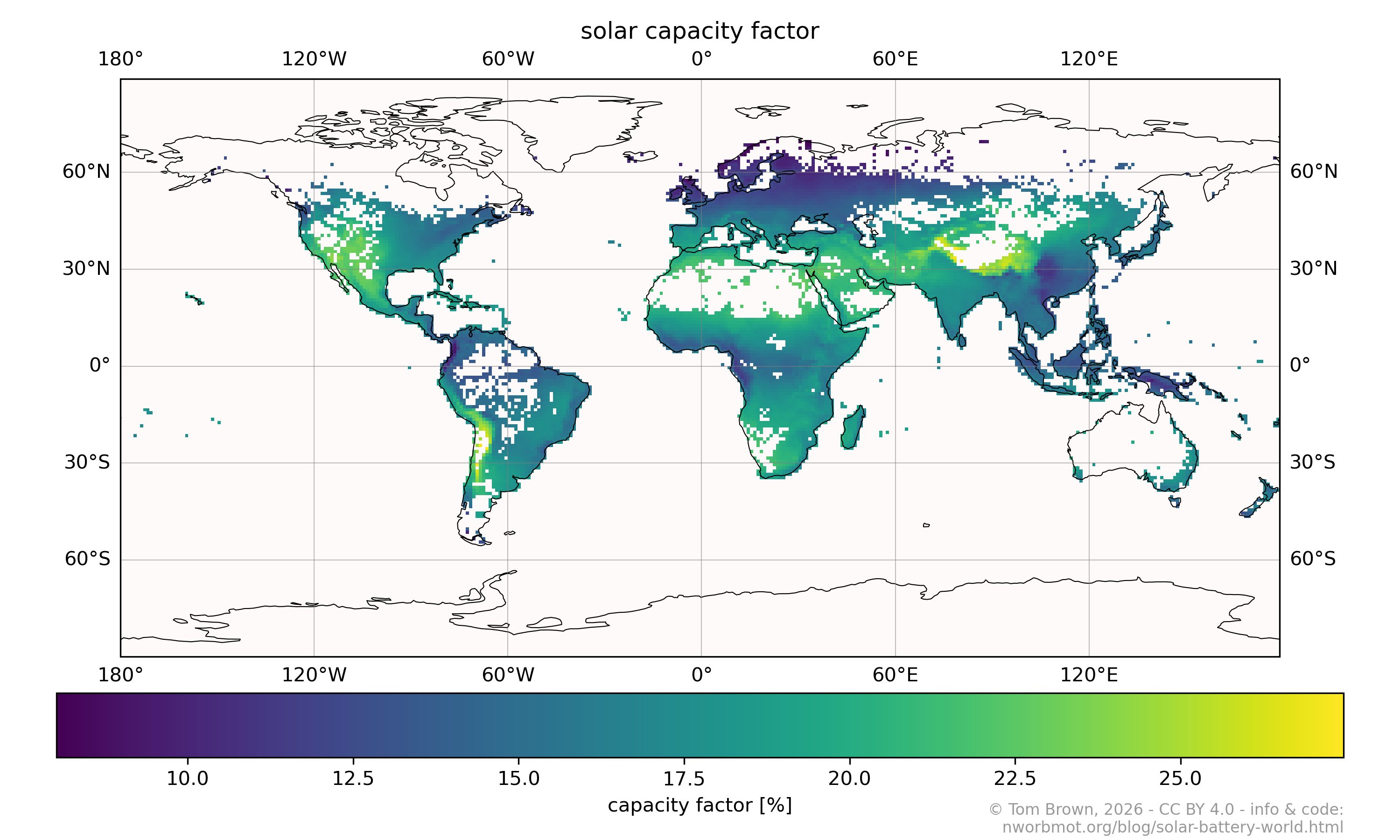
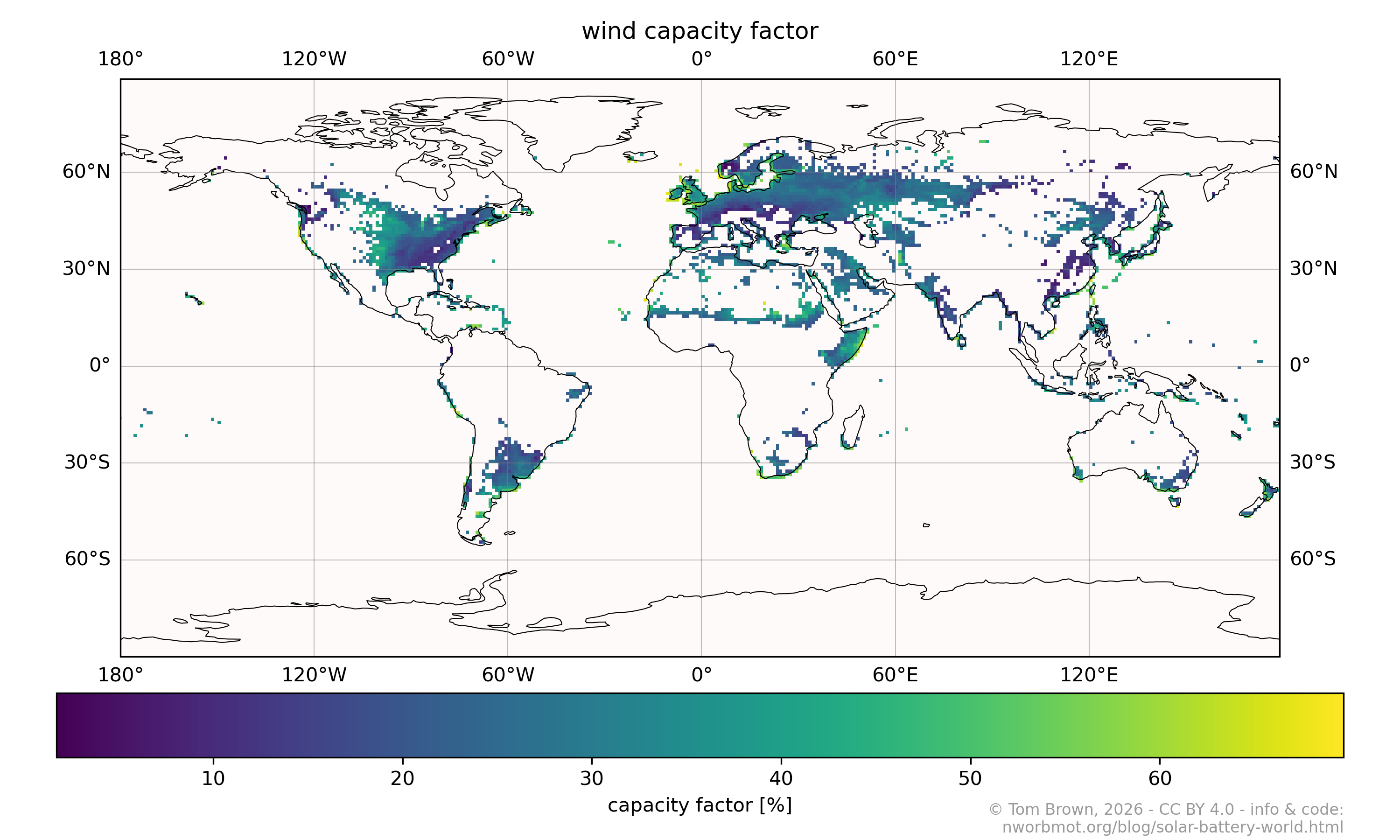
Here are the capacity factors (average production divided by capacity)
for solar and wind, at the locations where they are built by the model:

The setup is somewhat similar to a 2025 Ember report, but whereas they
fixed the solar and battery capacities relative to a constant demand,
and varied the location, we fix instead the fraction of load supplied,
and optimise the solar and battery capacities.

Victoria et al, 2021 also pointed out the coincidence of low seasonal
solar variation and the locations where most of the population lives
in this nice graphic: