Reverse-engineering the vintage Intel 8087’s tangent algorithm: more than CORDIC

I hope you’re not tired of the 8087, because I have another article about
Intel’s floating-point chip.1
In 1980, Intel introduced the 8087, making floating-point operations much faster
in the IBM PC and other systems.
In this article, I look at the algorithm behind the chip’s tangent instruction.
One popular approach for trigonometric functions is an algorithm called CORDIC.
Another approach is a polynomial approximation. The 8087 combined the two
to obtain both high accuracy and high performance.
The 8087 provided an enormous speedup over the 8086 microprocessor, computing a tangent in
90 microseconds rather than 13,000 microseconds.2

By examining the circuitry and microcode of the 8087,
I can explain the algorithm behind the tangent instruction, called FPTAN.
To explore the 8087’s circuitry, I popped the lid off a chip with a chisel
and created a high-resolution image with a microscope.
The microcode ROM is the large rectangular region in the center of the die, holding the 1648 micro-instructions that control the chip.
The bottom half of the chip (red box) is the datapath, the circuitry that performs floating-point calculations on 80-bit values.3

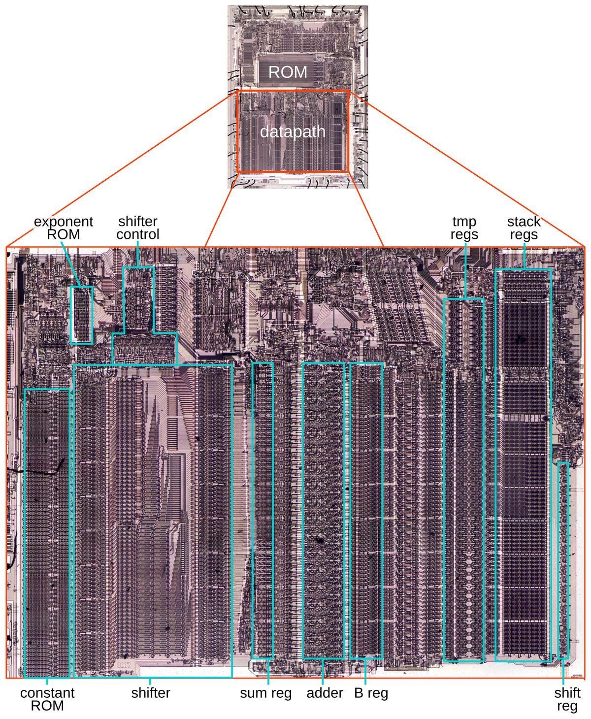
A close-up of the 8087’s datapath, showing functional blocks that are used by FPTAN. Click this image (or any other) for a larger version.

Zooming in on the datapath shows the relevant functional units.
The exponent ROM holds fixed exponent values that the algorithms need.
The constant ROM holds constants, including the constants used by the CORDIC algorithm.
The shifter is a large component; it shifts a 64-bit value left or right by arbitrary amounts.
The adder is the heart of the 8087’s calculations; as well as providing addition and subtraction, it is used in a loop for multiplication, division, and square roots.
The B register holds one input to the adder, while multiple sources can provide the other input. The sum register holds the adder’s output.
The eight stack registers and the temporary registers hold floating-point numbers.
Finally, the shift register holds 16 status bits for the CORDIC calculations.

The CORDIC algorithm

CORDIC is a clever algorithm for quickly computing transcendental functions
with simple hardware: it uses shift and add instructions along with table lookups,
but doesn’t need multiplication or division.
This algorithm dates back to 1956, when it was developed for the B-58 Hustler,
the first bomber capable of flying at Mach 2.
The aircraft had an analog navigation computer, but analog components provided limited accuracy.
Engineer Jack Volder was given the task of designing a digital computer to replace
the analog computer.7
One key problem was that an analog computer can easily generate sines and cosines
with an electromechanical device called a resolver.
But trigonometric functions are difficult to produce digitally, especially with the
slow transistors of that era.

Jack Volder came up with a fast way to calculate trigonometric functions
with simple hardware.
He called the algorithm—and the computer that implemented it—CORDIC: “COordinate Rotation DIgital Computer”.
CORDIC converts an angle to a vector, where
the vector’s coordinates provide the necessary trig functions.
The trick is to break down the angle into a sequence of special angles, angles that
make vector rotation easy.
These special angles are precomputed and stored in a table, so the CORDIC calculation
can be performed quickly, even on 1950s hardware.
Each CORDIC iteration provides an additional bit of accuracy, so the algorithm converges
rapidly. CORDIC became popular, including in scientific calculators, which used decimal CORDIC instead of binary.

Some trigonometry

I’ll try to keep the math to a minimum, but in this section I’ll give a quick explanation
of how CORDIC works.
The diagram below reviews how trig functions are related to the coordinates of a point.
Suppose you have an angle θ; it specifies a point (X, Y) on the unit circle.
The basic formulas are X=cos θ, Y=sin θ, and Y/X = tan θ.
Thus, if you can determine the coordinate (X, Y), then you can determine the value of the
trig functions.
If the point is not on the unit circle, e.g. (X’, Y’), then you can still easily determine
tan θ. (Spoiler: this is what the 8087 does.) However, sin θ and cos θ become messy.4

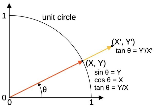
The relationship between an angle, the X and Y coordinates, and the trig functions.

If you’ve done any computer graphics, you’ve probably seen how a rotation matrix can rotate a point by an angle. (If you’re not familiar with rotation matrices, you can read about them here or just trust that it works.)
Multiplying a point (X, Y) by the rotation matrix yields the new point (X’, Y’) as shown below.

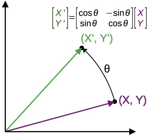
A point can be rotated by using a rotation matrix.

Unfortunately, since the rotation matrix (1, below) requires sin and cos, it doesn’t seem like it helps solve our problem.
However, we can divide the matrix by cos θ; this seems even less helpful since now the matrix (2) needs tan, which is what we want to evaluate. (Moreover, the vector’s length will grow.)
But the key to CORDIC is to use special angles, α_n = arctan(2^-n).
When we substitute one of these special angles into the matrix, we get matrix (3), which is easy to evaluate in hardware: multiplying by a power of 2 can be done by shifting the bits.

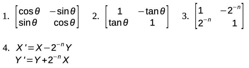
Simplifying the rotation matrix.

Applying matrix (3) to the point (X,Y) gives the equations (4).
These are key equations for the CORDIC process.
The important thing is that these equations are fast and easy to compute in machine language or
hardware, as the only operations are addition, subtraction, and binary shifting.

With that background, we can see how CORDIC works.
First, we break down the desired input angle into a combination of special angles that
adds up to the desired angle.5
Then we apply the rotation formula above for each special angle,
starting with the unit vector (1, 0). The result is a point
(X, Y) at the desired angle, and then the desired tangent is simply Y/X.6
Since the table of special angles is precomputed, the arctan operations don’t slow down the process.
As an aside, after the first few terms, the special angles approach 2^-n,
so they shrink by roughly a factor of 2 at each step.

To summarize, the CORDIC algorithm consists of looping through a table of stored angles.
If the stored angle is less than the desired angle, the stored angle is subtracted from the
desired angle to yield a new desired angle and the equations above (shifts, add, and subtract) are applied to yield a new vector.
At the end, the tangent of the original angle is given by Y/X.

The rational polynomial approximation

The accuracy of CORDIC depends on the number of terms that are used. With 16 terms, the
accuracy is approximately 2^-16, or 16 bits of accuracy.
To get 64 bits of accuracy would require calculating 64 terms (and a table of 64 special angles).
To get an answer faster, the 8087 uses 16 bits of CORDIC and uses another algorithm for
the remaining angle.
(The remaining angle is the gap between the sum of special CORDIC angles and the desired angle,
so it is very small, around 2^-16.)

For the remaining angle, the 8087 uses a Padé approximant, which is the ratio of two polynomials.
There’s a whole family of Padé approximations, depending on the order of the polynomials.
The 8087 uses a simple formula: 3x/(3-x²).8
Although this approximation is simple, it is very accurate for small values; its error is proportional to x⁴.
Since x<2^-16, the error will be less than 2^-64, meeting the 64-bit accuracy
requirement for the 8087.
Moreover, the 8087 doesn’t need to perform the division in the rational polynomial since
FPTAN returns a separate numerator and denominator. Thus, the division is “free”.

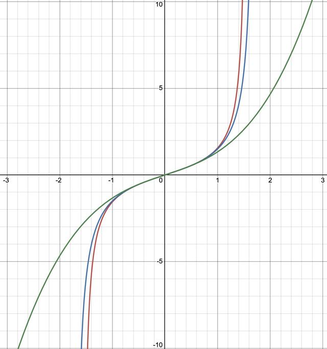
The tangent function (red), rational approximation (blue), and Taylor series (green).
Disclaimer: The Taylor series isn’t as bad as it appears, since the relevant range is very close to 0.
Graph generated with Desmos.

If you’ve studied calculus, you might think that a Taylor series polynomial is the way to go,
but the ratio of two polynomials is better.
(One reason is that tangent blows up to infinity at π/2.
A polynomial won’t blow up, but the ratio of polynomials can, so it fits the tangent function better.)
The graph above compares the tangent function (red), the rational approximation (blue),
and the third-order Taylor series (green).

Putting the pieces together: the 8087 algorithm

The 8087’s tangent algorithm has three parts: determining the CORDIC decision bits (called pseudo-division),
computing the rational approximation, and applying the rotation equations based on the
CORDIC decision bits (called pseudo-multiplication).9

In more detail, the first step determines which special angles to add to approximate the
input angle.
Each special angle is compared to the remaining input angle and subtracted if it is smaller.
If the angle is subtracted, a 1 is recorded; otherwise, a 0 is recorded.
Since this process is similar to how long division subtracts (or doesn’t subtract) successive
shifted versions of the divisor, generating 1s or 0s for the quotient, the process is known as pseudo-division.
Note that the rotations are not applied in this step. Instead, this step decides which rotations
to apply later.

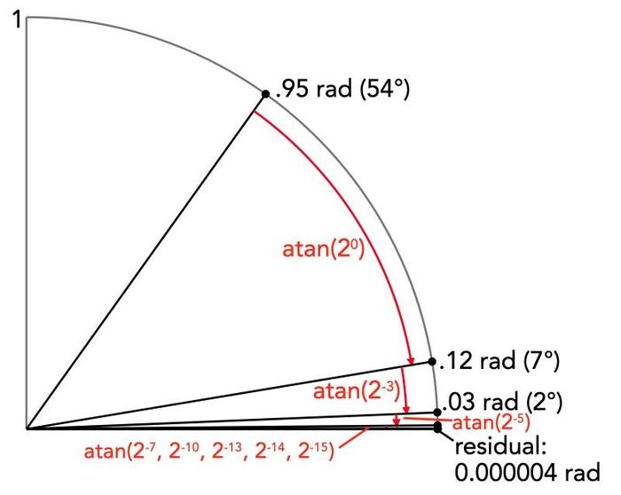
The diagram below shows this process applied to the input angle 0.95 radians.10
The process generates the sequence of bits
[1,0,0,1,0,1,0,1,0,0,1,0,0,1,1,1],
where the leftmost bit indicates arctan(2⁰) and so forth.
The angle is reduced by roughly a factor of 2 at each step, so the residual angle is
very small.

Next, the tangent of the remaining angle is calculated with the rational approximation
function, 3x/(3-x²).
The result is used as the initial vector for the next step.
The division is not performed here; instead, the numerator becomes Y in the initial vector
and the denominator becomes X. Thus, the expensive division step is avoided, since it
happens implicitly in the answer.
Multiplying by 3 is easy (shift left and add), so the only expensive operation at this
step is squaring the angle, which requires a full 64-bit multiplication.

The final step applies each CORDIC rotation if the corresponding decision bit from the first step is
1.
Since this is somewhat analogous to binary multiplication, which adds the multiplicand
at each step if the multiplier bit is 1, this step is known as pseudo-multiplication.
As described earlier, each rotation is computed with shifts, addition, and subtraction,
so each rotation is inexpensive.
Each rotation in this step corresponds to an angle reduction in the first step.
The rotations are applied in
reverse order—the smallest one first—to reduce rounding error.
To accomplish this, the decision bits are stored in a 16-bit shift register in the
first step, and shifted out in opposite order in this step.

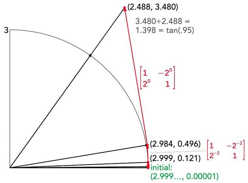
In the last phase of the CORDIC algorithm—pseudo-multiplication—a vector is rotated multiple times by applying shifts and adds. The final vector provides the tangent.

The diagram above shows the process applied to the input 0.95.
The initial vector (green) comes from the rational approximation function; it is very close to
(3, 0), but slightly rotated due to the tiny residual angle.
Each rotation step generates a new vector that matches the angle from the corresponding
step in the first part; I show two of the rotation matrices.
Note that the vectors diverge from the circle—a consequence of dividing each matrix by cos θ—but this doesn’t
affect the tangent.

The FPTAN instruction is somewhat peculiar as it doesn’t return the tangent directly.
Instead, it returns the Partial Tangent: the two coordinate values
(X and Y) that can be divided to produce the tangent.
One might wonder why the chip didn’t do the division automatically.
The motivation was that division
was slow back then, and omitting the division allowed for optimizations in some cases.

Relevant hardware details of the 8087

In this section, I’ll explain some features of the 8087 that are important for the microcode implementation of FPTAN.

The 8087 supports a variety of data types,
but internally, everything is stored as an 80-bit floating-point number called a “temporary real”.
A number has three parts: a sign bit, a 15-bit exponent, and a 64-bit significand (the fractional part),
In most cases, a floating-point number is represented by sign × significand × 2^exponent.
The advantage of floating-point numbers is that the exponent allows them to cover a huge range, from very small to very large.
The significand is a 64-bit binary number of the form 1.bbb…:
a leading 1, followed by the binary point (the binary equivalent of the decimal point) and the rest of the bits.11
One important detail is that the exponent is stored with a “bias” of 16383 added to it. Thus, the stored exponent is always positive, even if the real
exponent is negative. For instance, an exponent of 1 is stored as 0x4000, and an exponent of -16 is stored as 0x3fef.

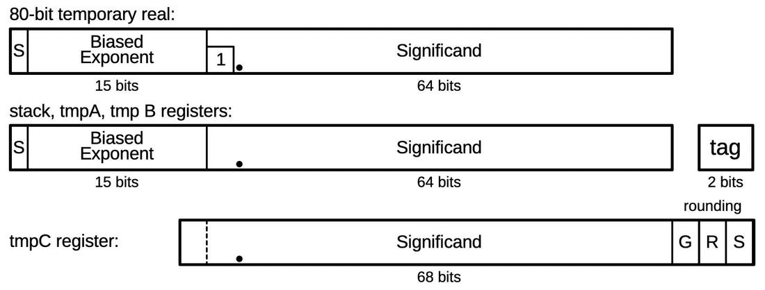
The 80-bit temporary real format and the register formats. The dot indicates the binary point, analogous to the decimal point.

To use the 8087, a programmer stores values in its eight internal registers, organized as a stack. Each register holds an 80-bit floating-point number.
To optimize performance,
each value in the register stack also has an associated “tag” value:
zero, valid, special, or empty.
A value of zero is tagged as zero.
A “normal” floating-point value is tagged as valid. If the value is infinity, Not a Number (NaN), or a denormalized value,
then it is tagged as special.
Finally, an empty tag indicates that a register does not hold a value; this allows detection of
stack underflow (reading an empty register) or stack overflow (storing to a non-empty
register).

The 8087 also has temporary registers that it uses internally: tmpA, tmpB, and tmpC.
(These registers are heavily used for the tangent calculation.)
tmpA and tmpB are 80-bit registers, along
with two tag bits.
However, tmpC is different: it doesn’t have a sign, exponent, or tag.
Moreover,
the significand is 68 bits; tmpC has an additional
bit to prevent overflow and three additional low-order bits for rounding, known as
guard, round, and sticky.

In the microcode,
each 16-bit micro-instruction performs one low-level operation.
Many of the operations move data from one register to another.
Other operations provide conditional jumps, subroutine calls, and returns.
A bit shift operation takes two micro-instructions: the first moves a value to the shifter and
configures the direction and amount of shift. The second micro-instruction (which may be
a distance after the first) moves the result from the shifter to a destination.

Similarly, addition takes two micro-instructions. The first micro-instruction
specifies the first argument to add and selects various options such as
carry and rounding.
(For subtraction, an option complements the second argument.)
The second argument always comes from the B register, which confusingly is
unrelated to the tmpB register.
The second micro-instruction moves the result from the sum register to a destination.

Implementation of the tangent algorithm in microcode

In this section, I’ll discuss some highlights of the tangent microcode.
The listing below shows the 8087’s microcode, along with my comments.
Each line indicates a 16-bit micro-instruction.
The control flow is a bit complicated, so I’ve put a flowchart in the footnotes.12

FPTAN:
#1039 st(0) -> tmpA        store argument in tmpA
#1040 stackPtr--           check if room on stack to push result
#1041 stack overflow?
#1042 jmp #1022 if tmp empty/special/overflow/div exit if bad argument or stack overflow
#1043 jmp #1045 if tmpA:tag ZERO is argument 0?
#1044 except:precision     precision exception except for 0
#1045 expconst 0x3ff0      Test if exponent >= -16
#1046 adder: tmpA:exp + 0 cin=1 argument exponent + 1
#1047 expConst -> Breg
#1048 adder: sumreg:frac - Breg cin=1 subtract -15
#1049 jmp #1061 if adder pos CORDIC if exponent >= -16
#1050 expconst 0x3fff      non-CORDIC path:
#1051 tmpA:exp -> Breg     check original exponent
#1052 expConst -> tmpB:frac against exponent 0
#1053 adder: tmpB:frac - Breg cin=1 subtract
#1054 sumreg:frac -> expConv 3fff - exp (i.e. -exp unbiased)
#1055 sumreg:frac -> shiftcount
#1056 jmp #1082 if exponent[6:14] != 0 if exp > -64 goto rational approximation
#1057 high bit -> tmpB:frac otherwise return original argument
#1058 expConst -> tmpB:sign,exp push 1 for X (denom): result is orig angle
#1059 tmpB -> st(0)
#1060 RNI
#1061 expconst 0x0010      CORDIC path
#1062 sumreg:frac -> loopcounter loopcounter = exp + 16
#1063 tmpA:frac -> tmpC    tmpC = original angle
#1064 trig const -> Breg/rnd
#1065 adder: tmpC - Breg cin=1, roundmode subtract first CORDIC angle
#1066 adder sign -> cordic, shl save bit  in shift register
#1067 jmp #1079 if not adder pos
#1068 sumreg:frac,rnd -> tmpC
#1069 adder: tmpA:exp + 0 cin=1 increment exp if first angle used
#1070 sumreg:frac -> tmpA:exp
#1071 jmp #1079
#1072 shift tmpC L 0 bytes, 1 bits top of CORDIC scan loop
#1073 shift L -> tmpC      shift angle left
#1074 trig const -> Breg/rnd
#1075 adder: tmpC - Breg cin=1, roundmode subtract CORDIC angle
#1076 adder sign -> cordic, shl save decision bit in shift register
#1077 jmp #1079 if not adder pos
#1078 sumreg:frac,rnd -> tmpC
#1079 jmp #1072 if not const latch zero bottom of CORDIC scan loop
#1080 tmpC -> tmpA:frac    update tmpA, tmpB
#1081 expConst -> shiftcount 16 -> shiftcount (otherwise based on exponent)
#1082 tmpA:frac -> tmpB:frac Padé approximation
#1083 tmpA:frac -> Breg    tmpA = ang
#1084 call SQUARE          square the angle
#1085 shift sumreg:frac R count byte bit
#1086 shift R -> sumreg:frac shift twice to scale square
#1087 shift sumreg:frac R count byte bit
#1088 shift R -> Breg      Breg = ang^2
#1089 1.1 -> tmpB:frac     3 (with exp 1)
#1090 adder: tmpB:frac - Breg cin=0
#1091 sumreg:frac -> tmpB:frac tmpB (X) = 3-ang^2
#1092 shift tmpA:frac R 0 bytes, 1 bits
#1093 shift R -> Breg/rnd
#1094 adder: tmpA:frac + Breg cin=0, roundmode ang + ang/2
#1095 sumreg:sign,frac,rnd -> tmpC tmpC (Y) = 3×ang with appropriate exponent
#1096 expconst 0x3ff0      exponent -15
#1097 expConst -> Breg
#1098 adder: tmpA:exp - Breg cin=1
#1099 jmp #1118 if not adder pos skip if exponent too small
#1100 shift tmpC R 0 bytes, 1 bits CORDIC pseudo-multiplication path
#1101 #15 -> loopcounter
#1102 shift R -> tmpC
#1103 jmp #1113 if not cordic[0] CORDIC: if saved decision bit...
#1104 shift tmpC R loopcount send tmpC (Y) to shifter
#1105 tmpC -> Breg/rnd     send tmpC to adder
#1106 adder: tmpB:frac + Breg cin=0, roundmode tmpB (X) not shifted because tmpC scaled
#1107 sumreg:sign,frac,rnd -> tmpC tmpC = tmpC + tmpB (implicit >>n)
#1108 shift R -> sumreg:frac,rnd shifted old tmpC to sumreg
#1109 shift sumreg:frac,rnd R loopcount shift right again because tmpC scaled
#1110 shift R -> Breg/rnd  and send to B reg
#1111 adder: tmpB:frac - Breg cin=1, roundmode
#1112 sumreg:frac,rnd -> tmpB:frac tmpB = tmpB - tmpC>>n
#1113 cordic shr           shift out shift register bit
#1114 shift tmpC R 0 bytes, 1 bits start shift of tmpC (Y)
#1115 jmp #1118 if cordic==0 done if shift register empty
#1116 shift R -> tmpC      shift tmpC (Y) right
#1117 jmp #1103 if not const latch zero done if counter at zero
#1118 expconst 0x3fff      CORDIC done
#1119 tmpB:frac -> sumreg:frac Test top bit of tmpB (X)
#1120 jmp #1124 if reg bit 63 If set, use exponent 0
#1121 expconst 0x3ffe      Otherwise, use exponent -1 and
#1122 shift sumreg:frac L 0 bytes, 1 bits shift left one bit to normalize
#1123 shift L -> tmpB:frac
#1124 expConst -> tmpB:sign,exp store exponent in tmpB
#1125 tmpC -> tmpA:frac    store tmpC (Y) in tmpA
#1126 tmpC -> sumreg:frac,sign
#1127 jmp #1132 if not sumreg[64] test overflow bit
#1128 shift tmpC R 0 bytes, 1 bits if set, normalize by shifting right
#1129 shift R -> tmpA:frac
#1130 adder: tmpA:exp + 0 cin=1 and increment exponent by 1
#1131 sumreg:frac -> tmpA:exp
#1132 tmpB -> st(0)        tmpB to top of stack: X (denom)
#1133 stackPtr++
#1134 tmpA -> st(0)        tmpA to st(1): Y (numerator)
#1135 stackPtr--
#1136 RNI                  End of FPTAN

The FPTAN microcode starts at address #1039 (decimal).
The microcode starts by moving the argument from the top of the stack to the tmpA register.
If the top value is empty, this indicates a stack underflow. If the next element on
the stack (the position that will hold the result) is not empty, this indicates a stack
overflow. In either case, the microcode indicates an “invalid” exception and ends the instruction.

One peculiar feature of the 8087 is that it flags a result with a “precision” exception if
the result is not exact. (This happens very frequently, even for, say, 1/10.)
The only tangent that the 8087 can compute precisely is tan(0), so all other inputs
result in a precision exception (#1044).

Next, the argument’s exponent is tested, splitting the execution into three paths.
If the exponent is -64 or less, the argument is so small that
the tangent equals the argument, within the accuracy of the system.13
In this case (#1057), the original argument is returned unchanged (with the denominator 1 pushed), and the code ends.
The second case is if the argument’s exponent is -17 or less. In this case,
the CORDIC step is skipped, and the routine jumps directly to the rational approximation (#1082).

CORDIC pseudo-division

The most interesting case is the CORDIC path (#1061), taken if the exponent is between -1 and -16.
Conceptually, the code performs 16 CORDIC steps, using 16 stored angles.
However, the code is optimized, skipping the large angles for smaller
inputs.
Specifically, the loop counter is initialized based on the
exponent of the input angle (#1062).
The CORDIC pseudo-division loop (#1061–#1080) tests the angles, subtracting ones that aren’t too big.14

The decision results are recorded in a 16-bit shift register, located on the far right side of the die.
Presumably, this is where the layout had some unused space.
Since the shift register is loaded and unloaded serially, it doesn’t need access to the
internal fraction bus, just two lines to shift the bits in and out, so the shift
register could be located in otherwise unused space.

The code is optimized to use 64-bit integer arithmetic rather than floating-point arithmetic.
This makes it tricky to understand the code since values
must be viewed more as fixed-point numbers with
implicit exponents.
These exponents are not stored anywhere, but can be determined by analyzing the algorithm.
Even the angle constants in the ROM do not have explicit exponents.15
Moreover, the implicit exponents change for each step through the loop to preserve accuracy.
Roughly speaking, each cycle of the loop reduces the values by a factor of 2, and the
angle constants shrink accordingly.
If the values had a fixed exponent, they would end up with 16 leading zeros, wasting
precision. But by scaling the values each cycle (with a left shift),
the numbers continue to use the full 64 bits.
In other words, the hardware is performing fast integer arithmetic, but mathematically
you can think of it as fixed-point with exponents that don’t physically exist in the chip.
See the table in the footnotes16 for details on how the implicit exponents change through
the loop.

Rational polynomial approximation

After the CORDIC pseudo-division loop, the microcode calculates the rational polynomial
approximation (#1082).
The small-angle path rejoins the execution flow here.
The microcode to calculate the polynomial approximation has a few interesting features.
The most time-consuming part is the SQUARE routine, which multiplies a fixed-point number by itself.
Multiplication is complicated, so I’ll give the details in a later post.
But in brief, the 8087 uses Booth’s Algorithm to
multiply by two bits at a time (radix 4), so it is twice as fast as regular binary
multiplication.
The loop to perform the shifts and adds is implemented in hardware, rather than microcode.
That is, one microcode instruction performs 32 additions: the hardware tests the
bits, does the appropriate add or subtract, updates the loop counter, and loops.
For performance, the shifting is done with specialized shifters, not the 8087’s general-purpose
shifter.

Except for the square, the polynomials are calculated with additions rather than multiplications.
The constant 3 doesn’t come from the constant ROM, but from special-purpose transistors that
set the top two bits of the significand; this is usually used to supply an NaN.
(If the implicit exponent is 1, this corresponds to 3.)
Subtracting the square yields the numerator. For the denominator, the angle is shifted
right (i.e. divided by 2) and added to itself.
This performs a multiplication by 3 (technically by 1.5, but increasing the implicit
exponent to 1 turns this into 3).
It would be expensive to divide the numerator by the denominator; instead, the numerator
and denominator are used as the initial Y and X values for the following CORDIC steps.

CORDIC pseudo-multiplication

Next is the CORDIC loop where the rotations are applied to the vector (#1100).
The rotations are applied in the reverse order from how they were computed in the first step:
the smallest rotations are applied first to preserve accuracy.
Bits are shifted out of the shift register to indicate if the rotation should be applied or
not. As soon as the shift register is all zeros, the loop stops.
In other words, smaller angles go through the loop just a few times, not the full 16 times.

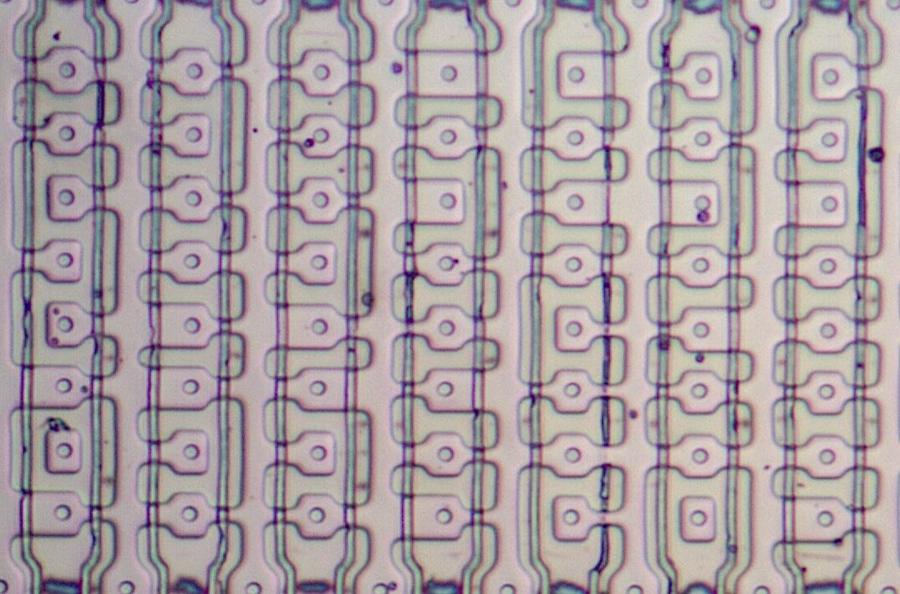
A close-up of the microcode ROM under the microscope. A transistor is formed where a vertical polysilicon line crosses doped silicon (pink). The 8087’s ROM is unusual: it uses four transistor sizes, so it stores two bits per transistor, twice the density of a regular ROM.

The rotations are applied by shifts and adds (or subtracts), but keeping track of the
implicit exponents is a bit tricky.
Since the vector starts almost horizontal, the X value is approximately 3, and the Y value
is around 2^-16.
As the vector rotates, X remains roughly 3, but Y potentially increases by a factor of 2
each time.
To provide the maximum accuracy for each number,
the exponent for X (tmpB) is 1, while the exponent for Y (tmpC) starts off at
-14 and increases by 1 each loop as Y is shifted right.
(Remember that these exponents are not stored anywhere but are implicit.)
Since the two registers have different (implicit) exponents, the values must be shifted
before adding.
The shift amounts aren’t intuitive; the table16 in the
footnotes may help clarify.

After the CORDIC loop,
the final part of the code (#1118) normalizes the X and Y values, creating the floating-point
values that are returned from the instruction.
Recall that these aren’t “real” floating-point values at this point, so they
may need adjustment.
Specifically, if X doesn’t have a
leading 1, it is shifted left one position, while if Y has two leading digits, it
is shifted right one position. In either case, the exponent is adjusted accordingly.
The X and Y values are put on the stack (#1132) to complete the instruction.

Conclusions

The FPTAN instruction is fairly slow as 8087 instructions go, due to its complexity.
The documentation says that it takes typically 450 clock cycles.
(The time has a large range; depending on the value, it can take 30 to 540 clock cycles.)
For the value I examined (0.95), 33% of the time is in the CORDIC
pseudo-division, 15% in the rational polynomial (mostly the squaring operation), 47% in the CORDIC pseudo-multiplication, and 5% overhead.

CORDIC is a popular way to compute trig functions, but there are alternatives such as polynomials.
The 8087 is unusual because it combines CORDIC and a rational polynomial.
For the Pentium, Intel moved from CORDIC to polynomial approximations;
the Pentium’s fast multiplication circuitry made polynomials practical.
Nowadays, Intel has libraries such as MKL (Math Kernel Library)
and
Short Vector Math Library (SVML) that provide highly optimized implementations tailored
to Intel hardware. These libraries are said to use polynomial approximations,
using parallel instructions (SIMD) for performance, rather than specialized hardware.
With these libraries, x87 operations and 80-bit floats are mostly obsolete.
Nonetheless, I hope you’ve enjoyed this look at an original 8087 algorithm.

I plan to continue reverse-engineering the 8087 microcode;
for updates, follow me on
Bluesky (@righto.com),
Mastodon (@[email protected]),
or RSS.
I’ve been working on this with the members of the “Opcode Collective”, especially Smartest Blob and Gloriouscow, who converted the
ROM images to microcode data and extensively analyzed the contents.
See the 8087 repository on GitHub for more.
AI statement: Despite the presence of the em dash, no AI was used in the writing of this article (details). The Opcode Collective used an ML algorithm to classify each ROM cell to extract the microcode.

Notes and references