the two kinds of random

Disclaimer: no AI was used to write this. Any errors, awkward sentences, and weird tangents are 100% organic, free-range, and human-made.

Picking up a puzzle I left lying around

Last post, right at the end, I dropped a puzzle and walked away from it. Here it is again, because this whole post is basically me refusing to let it go.

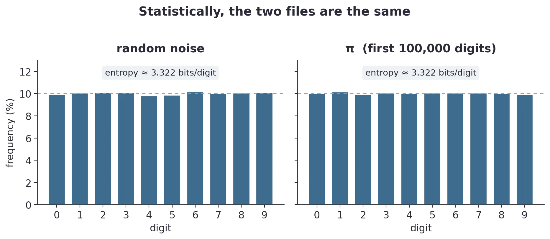
Imagine two files, and each one holds a million digits. The first one is pure noise — imagine I rolled a ten-sided die a million times and wrote down the results. The second one is the first million digits of $\pi$.

Now look at them the way a statistician would: count how often each digit from $0$ to $9$ shows up. In both files, every digit appears about a tenth of the time, so if you plot the two histograms you cannot tell them apart — both flat, both featureless. And you can run any “is this random?” test you like, because both files will pass. By every statistical measure, these two files are the same: both look like pure, incompressible randomness.

And yet.

One of these files I can send you in three lines. I write you a tiny program — “compute $\pi$, print a million digits” — and you regenerate the file exactly. The other file I cannot shrink at all, and to send it to you I have to send the whole thing, digit by digit, because there is no shorter description of it than itself.

So here is the entire post in one question:

If the two files are statistically identical, why can I compress one and not the other?

The thing is, this question does not have a simple answer, and I think that is exactly what makes it interesting. To get anywhere with it, we have to be careful about what the word “compressible” actually means — and once we are careful, it splits into two very different ideas. Most of this post is about pulling those two apart, and about a surprise waiting at the end of the second one: a kind of compressibility that you can always confirm when it is there, but can never rule out when it is not.

Two kinds of compression

One thing I want to be clear about from the start: everything in this post is about lossless compression, which means nothing is thrown away and nothing is approximated — I send you a shorter description, and you rebuild the exact original from it, bit for bit.

Even with that strict rule, I think there are really two different reasons a thing can be compressible, and this post is mostly about learning to tell them apart.

The first reason is statistical. Some symbols appear more often than others, so you give the common ones short codes and the rare ones long codes, and on average you save space. This is what zip files and Huffman coding do, and I think it is the kind of compression most people have in mind when they hear the word.

The second reason is about the process. The thing might come from a simple rule — a short program — even when its symbols look perfectly evenly spread out. In that case there is no statistical redundancy to exploit at all, and yet the thing still compresses, because the shortness lives in the process that generates it, not in the frequencies of its symbols.

So the real question of this post is: is statistical redundancy the only kind of compressibility there is? And $\pi$ is about to say no.

The statistical kind: entropy

Building entropy from a budget

Before we can say what is strange about $\pi$, we need to pin down what “statistical compression” even measures, and the measure has a name: entropy.

Informally, entropy is the average amount of surprise in a source of symbols. If a source always emits the same symbol, there is no surprise at all — you already know what is coming, so each new symbol tells you nothing, and the entropy is zero. If a source emits ten different digits with equal probability, every new symbol is as surprising as it can be, and the entropy is maximal. Most sources live somewhere in between: some symbols are common (little surprise, little information) and some are rare (big surprise, more information), and entropy is the average over all of them, weighted by how often each one shows up.

The connection to compression is direct: surprise is exactly the thing you have to pay bits for. Whatever is predictable you can leave out, because the receiver can fill it in, and whatever is surprising you have to actually transmit. So the entropy of a source, measured in bits per symbol, is the size of the shortest average message you can ever hope to achieve — it is the floor that no lossless code can go below.

That is the informal picture. But I don’t want to just state the formula and move on, because there is a way to actually derive it, and I am borrowing the spirit of it from Chris Olah’s lovely Visual Information Theory — the pictures below are my own version of his argument.

Here’s the setup. I want to send you a stream of symbols using as few bits as possible, by giving each symbol a codeword — a little string of bits. Common symbols should get short codewords; rare symbols can afford long ones, since I’ll rarely send them. That’s the whole intuition and it’s obviously right. The real question is: exactly how short, for a symbol that appears with probability $p$?

Here’s the catch that turns it into a real question. Codewords compete. To decode a stream unambiguously, no codeword can be a prefix of another — if 0 is a codeword, nothing else may start with 0. So handing out a short codeword is expensive: it eats a big chunk of the space of codewords still available. Precisely, a codeword of length $L$ costs a $1/2^L$

Think of it as a fixed budget. Every symbol has to buy a codeword, and short codewords cost more.

So how do you spend a fixed budget across your symbols? The natural move — and it turns out to be the optimal one — is to spend on each symbol in proportion to how often you use it: give a symbol of probability $p$ a $p$-sized slice of the budget. A slice of size $p$ buys a codeword of cost $p$, i.e. $1/2^L = p$

$$L = \log_2\frac🔥💬.$$

And there it is — not asserted, but derived. The ideal length of a codeword for a symbol of probability $p$ is $\log_2(1/p)$

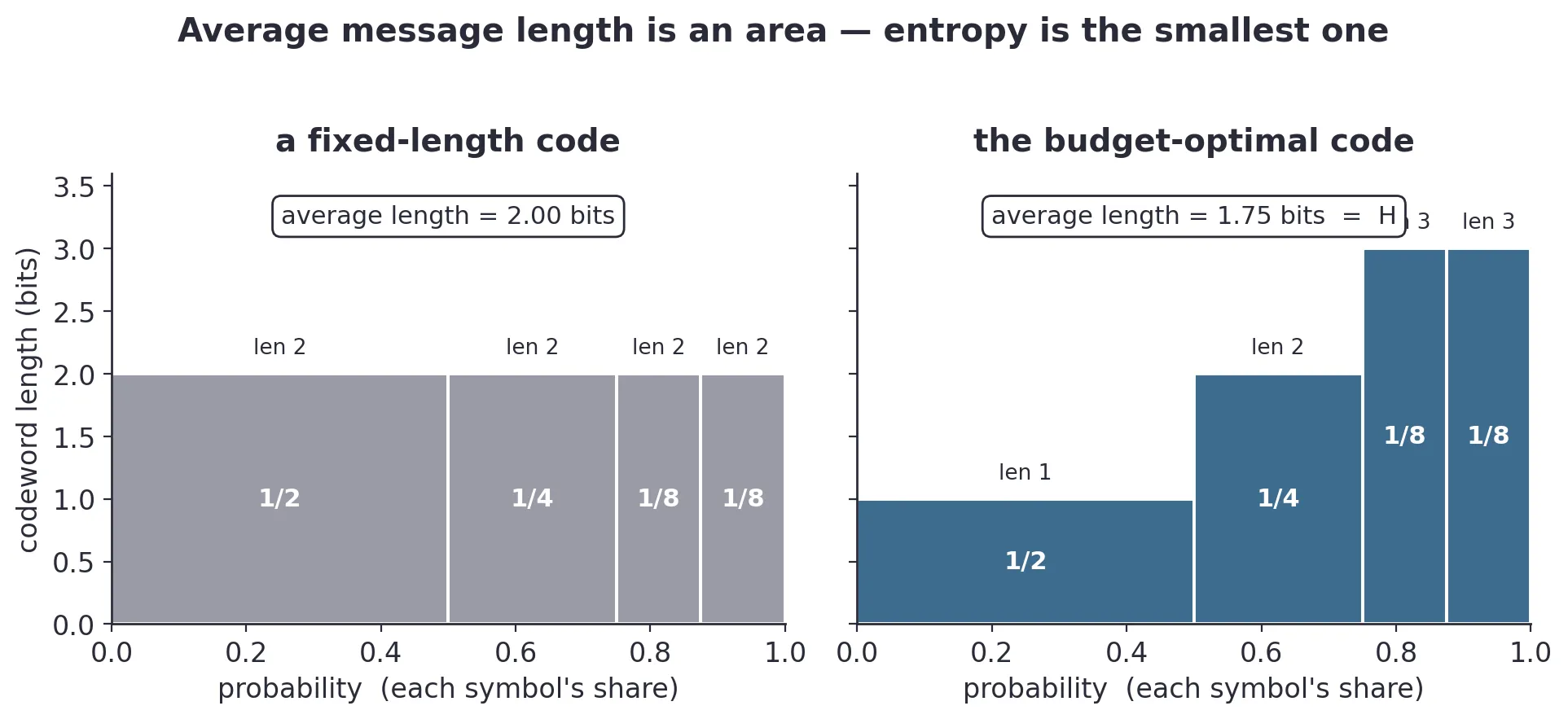
And here is the part I like most: you can see the average message length as an area. Put each symbol’s probability on one axis and its codeword length $\log_2(1/p)$

$$H = \sum_i p_i \log_2\frac🔥⚡ \;=\; -\sum_i p_i \log_2 p_i.$$

That is Shannon entropy, and it is the smallest possible area — the shortest average message any code can achieve for this distribution. If you give a common symbol a long codeword you add a lot of area, and the budget rule is exactly what removes that waste.

(There is a second way to read $\log_2(1/p)$

To feel it on a clean case, take four symbols with probabilities $\tfrac12, \tfrac14, \tfrac18, \tfrac18$

And here is the fact our puzzle needs: entropy is largest when everything is equally likely. A uniform distribution over ten digits maxes out at $\log_2 10 \approx 3.32$

Entropy’s blind spot

Now I want to show what entropy cannot see.

Entropy looks only at the distribution of symbols — how often each one appears. It never looks at their order, and it never looks at whether there is a rule generating them. You can take any structured sequence and shuffle it: the histogram does not change, so the entropy does not change, but you have destroyed whatever pattern a program could have used. Entropy did not notice anything, because it never saw the pattern in the first place.

And that is the crack $\pi$ slips through. Its digits have maximal entropy because, symbol by symbol, they are uniform. But $\pi$ is not made by rolling dice. $\pi$ is made by a rule — a short, fixed, deterministic rule that a program can carry out — and entropy is blind to that rule, because the rule leaves no fingerprint in the digit frequencies.

So we need a second notion of compressibility, one that can see rules.

The process kind: Kolmogorov complexity

Here it is, and it is very simple:

The Kolmogorov complexity $K(x)$ of a string is the length of the shortest program that outputs it.

Not the average of anything, not a distribution — one string, one shortest program.

A string of a billion zeros has tiny complexity, because print "0" a billion times is a very short program. A truly random string of length $n$ has complexity of about $n$, because no description is shorter than the string itself, so the “program” is basically “print the whole thing”. And $\pi$? Tiny — a couple hundred bits, because a small program grinds out its digits forever.

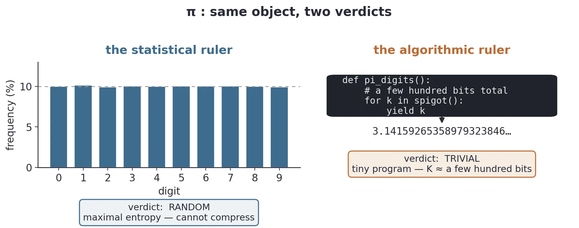
So the puzzle resolves, and the resolution is that we were holding two different rulers:

• Shannon entropy is statistical. It is about an ensemble — a source, a distribution, the long run — and it sees frequencies, nothing else.
• Kolmogorov complexity is structural. It is about one object, and it sees rules, structure, generating processes.

$\pi$ is the object where the two rulers disagree as loudly as possible: maximal entropy, minimal complexity. Statistics says “random, cannot compress”, and Kolmogorov says “trivial, here is a five-line program”. Both are right, because they are answering different questions.

There is a bridge between the two, though: for a truly random source, the expected Kolmogorov complexity of its outputs equals its Shannon entropy, up to a small constant. So on average, over a whole distribution, the two rulers agree, and I like to think of statistics as the shadow that algorithmic structure casts when you only look at ensembles. The two only come apart for individual, special objects that hide a generating rule, and $\pi$ is the extreme case of that. But most objects are not special at all — and that is the next thing, because it is the one thing here that you can actually prove.

Almost nothing can be compressed

Here is a claim that sounds hard and is actually a subtraction:

Almost every string is its own shortest description. Most things cannot be compressed at all.

Watch. Fix a length $n$ and ask: how many strings of length exactly $n$ are there? Two choices per position, $n$ positions, so $2^n$

Now ask: how many possible descriptions are shorter than $n$ — that is, programs of length $0, 1, 2, \dots, n-1$

$$1 + 2 + 4 + \dots + 2^{\,n-1} = 2^n – 1,$$

which is one fewer than the number of strings.

That is the whole argument. There are $2^n$

And if you push the same counting a little further, the situation gets much worse. Suppose you want real compression, a description at least $c$ bits shorter. There are only about $2^{\,n-c}$

There is something about the shape of this argument that I want to point out, because it comes back again later: we just proved that incompressible strings are almost all of them without ever naming a single one. It is like counting doors and counting keys and realizing there are not enough keys — we know some door has to stay locked, but the counting never tells us which one, because we never actually opened any door.

There is also a move hiding inside the counting that is worth saying out loud: a program is itself a string. This is the only reason we could put “number of strings” and “number of programs” side by side and subtract, because they are the same kind of object, measured in the same bits. I think this simple fact is what the rest of the post depends on, so hold onto it.

One more thing this counting settles. When I first understood this argument, I tried to be clever and dodge it. What if I don’t store the string itself, but its index in the list of all strings? Or what if I write a short program that generates many strings from a seed, and I just store the seed? It turns out every scheme like this fails in the same way, and the reason is always the same:

To select one specific thing from a family of size $N$, you need a name that can tell $N$ things apart, and a name that distinguishes $N$ possibilities costs about $\log_2 N$

An index into $2^n$

Everything so far is provable just by counting, and it is solid ground. But the moment we stop counting and try to actually find these shortest descriptions, the ground gives way.

The catch: you can never compute it

The definition of Kolmogorov complexity is clean and simple, but there is a catch that I find genuinely strange the first few times you meet it: you can never actually compute it. There is no algorithm that takes a string and hands you back its complexity.

The reason comes down to an asymmetry that I think is worth sitting with, so let me try to spell it out slowly.

First, think about what you can do. You can go looking for short programs, and if you happen to find one of length 50 that prints your string, then you have proven that $K(x)$ is at most 50 — the program is sitting right there, you run it, and it works. And you can keep looking, so maybe tomorrow you stumble onto an even shorter one. This means your upper bound on the complexity can always come down, and you can always discover that a string is simpler than you thought it was.

Now think about the opposite direction, where you want to certify that $K(x)$ is at least 50 — that no program shorter than 50 prints your string. This is no longer a claim about one program, it is a claim about all of the shorter programs at once. And to rule out even a single one of them, you would have to run it and watch what it does, but it might run for a billion steps and then suddenly print your string, or it might run forever without ever stopping, and you can never be sure which of those two is going to happen. So you can never close the case on even one candidate, let alone all of them at once, which means the lower bound stays sealed.

Upper bounds are findable, but lower bounds never are. You can always learn that a thing is more compressible than it looked, but you can never certify that it is as incompressible as it looks.

And there is a sharper version of this, which is that $K$ is not just hard to compute but uncomputable outright, and it comes from a paradox that you probably already know in its everyday form. Think about the phrase “the smallest number not describable in fewer than twelve words.” There are only finitely many phrases with fewer than twelve words, so only finitely many numbers can be pinned down that way, which means some numbers must escape being described at all — and among those, there has to be a smallest one. But now look at the phrase again: it just named that number, using only eleven words. So the number both can and cannot be described in fewer than twelve words, which is a contradiction. This is the Berry paradox, and here is how it turns into a real theorem. Suppose that some algorithm could compute $K$ for us. Then I could write a short program that says: “go through the strings in order, and print the first one whose complexity is greater than a billion.” That program is short — a few thousand bits is enough — and yet the string it prints is one that it just certified as needing more than a billion bits to produce. So that string somehow has a few-thousand-bit description (the program itself) and a billion-bit complexity at the very same time, which cannot be. The only thing we assumed was that $K$ is computable, so that assumption must be the thing that is wrong.

Notice that this argument never once ran a program and waited around to see whether it would halt. It is pure self-reference: if you could measure complexity, then you could write a short program that names something complex, and that is already a contradiction. Self-reference is what makes the whole thing work, and self-reference is only possible because a program is itself a string, one that other programs can read and search through and run. Which is exactly the same fact we leaned on in the counting argument — a program is a string — quietly doing the work again.

What this was really about

Underneath the whole thing, I think there is a single distinction, and it is the real subject of this post. It is the difference between two kinds of statement:

• “There are $N$ things.” This is a statement about the size of a set. It does not tell any of them apart, and precisely because it does not differentiate, it is cheap — it carries almost no information.
• “This is the $K$-th thing.” This is a statement that singles one out, and to do that among $N$ possibilities costs about $\log_2 N$

Almost everything we ran into is that gap. “Most strings are incompressible” is a headcount — cheap, and provable just by counting. “This string is incompressible” is a roll call — and the roll call is exactly the thing we could never do. It showed up one more time in the asymmetry between finding and ruling out: you can always find a short program if one exists, because that is a single witness and you reach it in finite time, but you can never rule out all the shorter ones, because that is a claim about the whole infinite set at once. Finding one is finite; settling all of them is not.

And it loops right back to entropy, because what is information, really? It is the cost of telling things apart:

$$\boxed{\ \text{selection cost} \;=\; \log_2(\text{number of things you must tell your target apart from})\ }$$

Entropy is the average of that cost over a distribution, and Kolmogorov complexity is that same cost for one specific object, so both are really asking the same thing: which one, out of how many. Compression, then, is just everything you don’t have to select. $\pi$ compresses to almost nothing because, once its little generator is running, there is nothing left to point at — no choice to pay for. A random string compresses to nothing because you have to point at all of it, every single bit. Both kinds of compression, the statistical and the structural, turn out to have the same price: the price of differentiation. And the cheapest possible statement is the one that differentiates nothing at all — there are $N$.

Where this goes next

I am stopping here on purpose, because this post was really about one question — why I can compress $\pi$ and not its statistical twin — and I would rather it do that one thing well than wander. But the same accounting keeps going, and there are a few places I want to take it later.

When compression becomes learning. Everything here was lossless, but there is a lossy version of the same idea — the shortest program for something only approximately like your data, one that keeps the structure and throws away the noise — and that turns out to be more or less what learning is. Occam’s razor stops being a slogan and becomes arithmetic: the best explanation is just the shortest program that still fits.

When you can’t even prove it. The counting argument tells us almost every string is incompressible, but it never hands us a single specific one, and it turns out that is not a temporary gap we might close with a clever idea. There is a point where this stops being about computers and starts being about the limits of proof itself — where a formal system simply cannot prove that any particular string is complex, no matter how true that is. That one runs straight into Gödel, and it deserves its own post.

The finite universe. If you only ever get to name physical things, and the universe holds only a finite number of distinguishable states, then all of this becomes finite — selection cost turns into $\log_2$

But those are their own posts. This one was about a single question, and the surprising place it led. You can always tell that $\pi$ can be compressed, by simply handing over the program — but for its random-looking twin, you can never be sure that it can’t be. You can find a short description whenever one exists, and you can never prove that none does.